Contents
%%%%%%%%%%%%%%%%%%%%%%%%%%%%%%%%%%%%%%%%%%%%%%%%%%%%%%%%%%%%%%%%%%%%%%%%%%%%%%%
% Name: test_compute_tempogram_autocorrelation.m
% Date of Revision: 2011-10
% Programmer: Peter Grosche
% http://www.mpi-inf.mpg.de/resources/MIR/tempogramtoolbox/
%
% Description: Illustrates the following steps:
%   1. loads a wav file
%   2. computes a novelty curve
%   3. computes an autocorrelation-based tempogram
%   4. visualizes the lag-axis tempogram
%   5. rescales to linear tempo axis
%
% Audio recordings are obtained from: Saarland Music Data (SMD)
% http://www.mpi-inf.mpg.de/resources/SMD/
%
%
% License:
%     This file is part of 'Tempogram Toolbox'.
%
%     'Tempogram Toolbox' is free software: you can redistribute it and/or modify
%     it under the terms of the GNU General Public License as published by
%     the Free Software Foundation, either version 2 of the License, or
%     (at your option) any later version.
%
%     'Tempogram Toolbox' is distributed in the hope that it will be useful,
%     but WITHOUT ANY WARRANTY; without even the implied warranty of
%     MERCHANTABILITY or FITNESS FOR A PARTICULAR PURPOSE.  See the
%     GNU General Public License for more details.
%
%     You should have received a copy of the GNU General Public License
%     along with 'Tempogram Toolbox'. If not, see
%     <http://www.gnu.org/licenses/>.
%
% Reference:
%   Peter Grosche and Meinard Müller
%   Extracting Predominant Local Pulse Information from Music Recordings
%   IEEE Transactions on Audio, Speech, and Language Processing, 19(6), 1688-1701, 2011.
%
%   K. Jensen
%   Multiple scale music segmentation using rhythm, timbre and harmony
%   Eurasip Journal on Advances in Signal Processing, Vol. 2007, 2007.
%%%%%%%%%%%%%%%%%%%%%%%%%%%%%%%%%%%%%%%%%%%%%%%%%%%%%%%%%%%%%%%%%%%%%%%%%%%

clear
close all


dirWav = 'data_wav/';

filename = 'Debussy_SonataViolinPianoGMinor-02_111_20080519-SMD-ss135-189.wav';
1., load wav file, automatically converted to Fs = 22050 and mono
%%%%%%%%%%%%%%%%%%%%%%%%%%%%%%%%%%%%%%%%%%%%%%%%%%%%%%%%%%%%%%%%%%%%%%%%%%%

[audio,sideinfo] = wav_to_audio('',dirWav,filename);
Fs = sideinfo.wav.fs;
2., compute novelty curve
%%%%%%%%%%%%%%%%%%%%%%%%%%%%%%%%%%%%%%%%%%%%%%%%%%%%%%%%%%%%%%%%%%%%%%%%%%%

parameterNovelty = [];

[noveltyCurve,featureRate] = audio_to_noveltyCurve(audio, Fs, parameterNovelty);
3., compute autocorrelation-based tempogram
important parameters: .tempoWindow: trade-off between time- and tempo resolution try chosing a long (e.g., 12 sec) and short (e.g., 3 sec) window .maxLag/.minLag: tempo range
%%%%%%%%%%%%%%%%%%%%%%%%%%%%%%%%%%%%%%%%%%%%%%%%%%%%%%%%%%%%%%%%%%%%%%%%%%%


parameterTempogram = [];
parameterTempogram.featureRate = featureRate;
parameterTempogram.tempoWindow = 6;                  % window length in sec
parameterTempogram.maxLag = 2;                    % corresponding to 30 bpm
parameterTempogram.minLag = 0.1;                  % corresponding to 600 bpm

[tempogram, T, Lag] = noveltyCurve_to_tempogram_via_ACF(noveltyCurve,parameterTempogram);
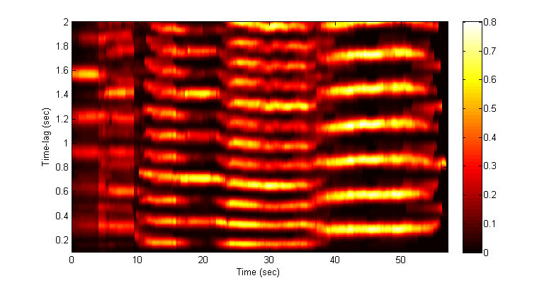
4., visualize with time-lag axis
%%%%%%%%%%%%%%%%%%%%%%%%%%%%%%%%%%%%%%%%%%%%%%%%%%%%%%%%%%%%%%%%%%%%%%%%%%%

parameterVis = [];
parameterVis.yAxisLabel = 'Time-lag (sec)';

visualize_tempogram(tempogram,T,Lag,parameterVis)
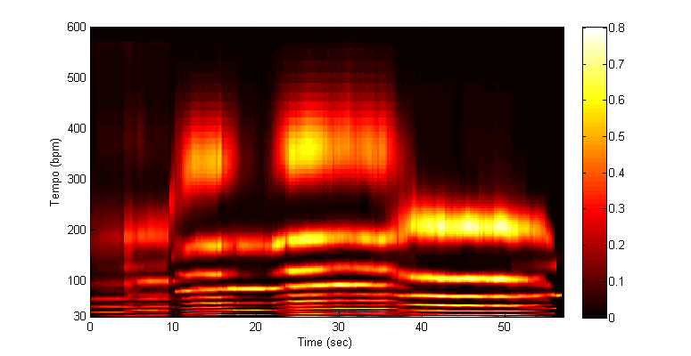
5., rescale to linear tempo axis
%%%%%%%%%%%%%%%%%%%%%%%%%%%%%%%%%%%%%%%%%%%%%%%%%%%%%%%%%%%%%%%%%%%%%%%%%%%

BPM_in = 60./Lag;
BPM_out = 30:1:600;
[tempogram,BPM] = rescaleTempoAxis(tempogram,BPM_in,BPM_out);

visualize_tempogram(tempogram,T,BPM)