3. Global Illumination Methods

3.1 Radiosity Methods

3.1.1-3 Radiosity for Lambertian Environments

Four stages of progressive image quality refinement using the hierarchical radiosity algorithm with clustering described in Sections 3.1.1-3.
 
 

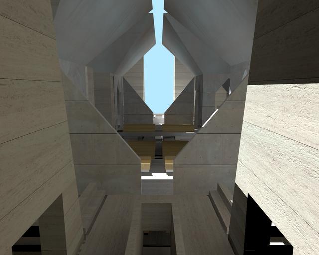
Radiosity solution for complex architectural environment using the techniques proposed in Sections 3.1.1-3.
 

3.1.4 Radiosity for Non-Lambertian Environments

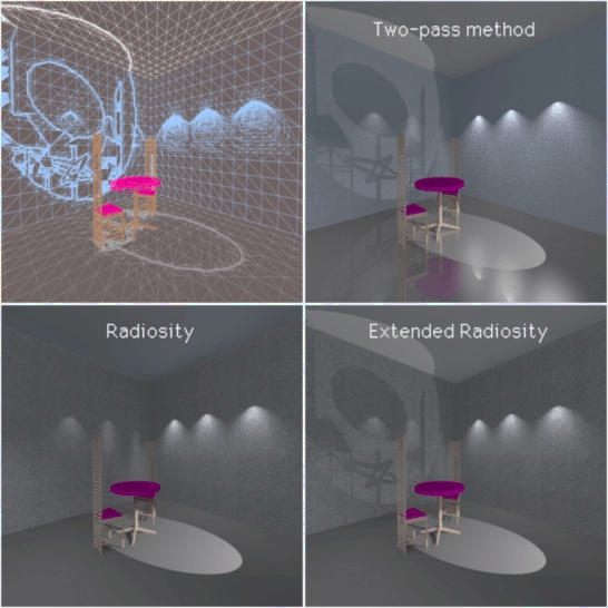
The "image method" used for primary lights. The bottom-left image was obtained using the traditional hierarchical radiosity algorithm described in Sections 3.1.1-3. The bottom-right image was obtained using the radiosity algorithm extended with the "image method" described in Section 3.1.4. The corresponding mesh used for the radiosity solution is shown in the top-left image. The top-right image was obtained using a hybrid of radiosity and ray tracing solutions discussed in Section 3.4.
 
 

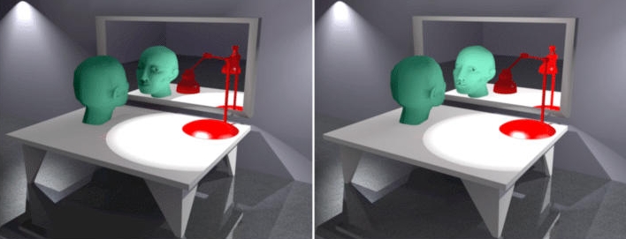
Clustering of secondary "virtual lights" for the image method. In the left image the mirror was ignored during the shooting radiosity iteration, while it was considered in the right image. Note the complex light path that was simulated in the latter case: the face is mostly illuminated by light emitted by the red lamp, which is reflected by the table and then by the mirror.
 
 
 

3.2 Stochastic Methods
 

3.2.4 Enhanced Density Estimation Methods

a)	b)

Figure 3.3: Enhanced density estimation methods: a) Plot of the RMS_error for the NN and ENN methods as a function of the number of nearest neighbors N_Max. For the NN method, the search of N_Max nearest photons is always performed for all lighting reconstruction points x_i. For the ENN method,   N_Max is the maximum number of nearest photons N_i^opt (corresponding to h_i^opt ) to be found for every point x_i. The numbers within the graphs show the total number of photons available for reconstruction of the lighting pattern shown in b).
 

1         10         100         1000

estimated  error

ENN method

actual error  for ENN

NN  method

actual error for NN

Comparison of illumination textures (IT) computed using the ENN and NN methods for the lighting pattern shown in Figure 3b. Also, the distribution of the estimated local error using equation (3.9), and the actual local error computed for every texel independently are shown (the average actual error values are depicted in Figure 3a as the RMS_error  plots).  The meaning of the images is as follows: distribution of the estimated error (the first column), illumination textures and the corresponding distribution of the actual error  for the ENN and NN methods (the second and third columns, and the last two columns, respectively). The rows of images correspond to an average number of  1, 10, 100, and 1000 photons per texel. Color scale for the locally measured relative reconstruction error is as follows: blue up to 10%, green up to 20%, red 20% and more. As can be seen the ENN method leads to smaller local error values and a better reconstruction of discontinuities in the lighting function than the NN method.
 
 

3.2.5 Density Estimation at Interactive Speeds
 

a)	b)

Figure 3.4: Excessive noise reduction at early stages of the Monte Carlo computation: results of lighting reconstruction for the scene built of 116,600 mesh elements after 10 seconds of photon tracing (Pentium II, 400 MHz processor) in two cases: a) without filtering, and b) with filtering.
 
 

3.4 Hybrid Methods

An example of animation  computed using a hybrid of the radiosity and ray tracing methods. Note that this animation is presented in the QuickTime format, which requires a specialized animation viewer supporting this format, e.g., QuickTime plug-in for web browsers available under the URL: http://www.apple.com/quicktime/.